This is version 1.0.0 of MoNAn. This update includes many changes, including some that mean old code written for older versions will not work anymore!
Code use has been simplified; the most important changes are:
the cache is now hidden from the user and does not need to be create or specified in functions anymore
there is a new way to specify the model with createEffects and addEffect
in gofMobilityNetwork there is no need to specify “simulations” anymore
new way to generate the process state using monanDataCreate
MoNAn is the software implementation of the statistical model outlined in:
Block, P., Stadtfeld, C., & Robins, G. (2022). A statistical model for the analysis of mobility tables as weighted networks with an application to faculty hiring networks. Social Networks, 68, 264-278.
Link to the study in Social Networks.
Pre-print with minor differences to the journal version.
The model allows for the analysis of emergent structures (known from network analysis) in mobility tables, alongside exogenous predictors. It combines features from classical log-linear models for mobility tables and Exponential Random Graph Models (ERGMs). In the absence of emergent structures, the models reduces to the former, when ignoring characteristics of individuals, it is an ERGM for weighted networks.
Announcements about workshops etc. can be found here.
The MoNAn Manual is available here on github in the manual folder or on SocArXiv
As of 30 Aug 2023, we have a CRAN release of the package. Nevertheless, the package and the documentation might still have bugs or errors, or you might not be able to do what you want. In that case, or if you are unsure please write the package maintainer under his institutional email address.
We are currently (Mar 2024) on version 1.0.0 on github. Version 0.1.3 was released to CRAN in Feb 2024.
You can install MoNAn either from CRAN or from GitHub.
The advantage of installing from github is that you will always stay up-to-date with the latest developments, in particular, new functionality and effects. You can install the current version of MoNAn from GitHub using:
However, you can also get the (often slightly older) CRAN version with:
In this section, we outline a simple example with synthetic data stored in the MoNAn package.
The example case uses synthetic data that represents mobility of 742 individuals between 17 organisations. The artificial data includes an edgelist, i.e., a list of origins (column 1) and destinations (column 2) of all individuals sorted by origin.
mobilityEdgelist[1:10,]
#>       [,1] [,2]
#>  [1,]    1    1
#>  [2,]    1    1
#>  [3,]    1    2
#>  [4,]    1    2
#>  [5,]    1    2
#>  [6,]    1    2
#>  [7,]    1    3
#>  [8,]    1    3
#>  [9,]    1    3
#> [10,]    1    3
The data further includes (artificial) characteristics of individuals, which we will call sex. However, using continuous covariates is also possible, although for some effects this would not be meaningful.
Characteristics of the organisations are the region in which they are located (binary, northern/southern island) and the organisations’ size that represents a composite measure of the number of workers, assets, and revenue.
orgRegion
#>  [1] 1 1 1 1 1 1 1 0 0 0 0 0 0 0 0 0 0
orgSize
#>  [1]  3.202903  5.178353  7.592492  7.368718  9.098950  7.977469  7.751859
#>  [8] 10.454544  7.811348  4.958048  7.740106  6.112728  6.640621  2.850886
#> [15] 8.955254 7.597493 9.313139First, we create MoNAn data objects from the introduced data files. A necessary part is that we define and name the nodesets, i.e., we name who (“people”) is mobile between what (“organisations”).
# extract number of individuals and organisations from the mobility data

N_ind <- nrow(mobilityEdgelist)
N_org <- length(unique(as.numeric(mobilityEdgelist)))

# create monan objects
people <- monanEdges(N_ind)
organisations <- monanNodes(N_org)
transfers <- monanDependent(mobilityEdgelist,
                            nodes = "organisations",
                            edges = "people")

sameRegion <- outer(orgRegion, orgRegion, "==") * 1
sameRegion <- dyadicCovar(sameRegion, nodeSet = c("organisations", "organisations"))

region <- monadicCovar(orgRegion, nodeSet = "organisations")
size <- monadicCovar(orgSize, nodeSet = "organisations")
sex <- monadicCovar(indSex, nodeSet = "people", addSame = F, addSim = F)
We combine the data objects into the process state, i.e., a MoNAn object that stores all information about the data that will be used in the estimation later. We must include one outcome variable (transfers) and two nodeSets (people, organisations).
myState <- monanDataCreate(transfers,
                           people,
                           organisations,
                           sameRegion,
                           region,
                           size,
                           sex)

# inspect the created object
myState
#> dependent variable: transfers with 742 people mobile between 17 organisations
#>
#> covariates of organisations
#>  cov. name    range    mean
#>  sameRegion    0-1     0.52
#>  region        0-1     0.41
#>  size       2.85-10.45 7.09
#>
#> covariates of people
#>  cov. name range mean
#> sex 0-1 0.53The predictors in the model are called “Effects”. To specify a model, first an empty effects object is created that only uses the state, and then effects are added one-by-one. Adding an effect requires the effects name and any additional parameters it needs.
# create an effects object
myEffects <- createEffects(myState)
myEffects <- addEffect(myEffects, loops)
myEffects <- addEffect(myEffects, reciprocity_min)
myEffects <- addEffect(myEffects, dyadic_covariate, attribute.index = "sameRegion")
myEffects <- addEffect(myEffects, alter_covariate, attribute.index = "size")
myEffects <- addEffect(myEffects, resource_covar_to_node_covar,
                       attribute.index = "region",
                       resource.attribute.index = "sex")
myEffects <- addEffect(myEffects, loops_resource_covar, resource.attribute.index = "sex")

# There is also a simpler way using pipes (|>) and using the more intuitive
# node.attribute & edge.attribute instead of the older
# attribute.index & resource.attribute.index:
myEffects <- createEffects(myState) |>
  addEffect(loops) |>
  addEffect(reciprocity_min) |>
  addEffect(dyadic_covariate, node.attribute = "sameRegion") |>
  addEffect(alter_covariate, node.attribute = "size") |>
  addEffect(resource_covar_to_node_covar,
            node.attribute = "region",
            edge.attribute = "sex") |>
  addEffect(loops_resource_covar, edge.attribute = "sex")

# inspect the created object
myEffects
#> Effects
#>  effect name                  cov. organisations cov. people  parameter
#>  loops                                -               -           -
#>  reciprocity_min                      -               -           -
#>  dyadic_covariate                 sameRegion          -           -
#>  alter_covariate                     size             -           -
#>  resource_covar_to_node_covar       region           sex          -
#> loops_resource_covar - sex -We can run a pseudo-likelihood estimation that gives a (biased) guess of the model results. We use this to get improved initial estimates, which increases the chances of model convergence in the first run of the estimation considerably. To get pseudo-likelihood estimates, we need to use functions from other libraries to estimate a multinomial logit model (e.g., “dfidx” and “mlogit”)
# create multinomial statistics object pseudo-likelihood estimation
myStatisticsFrame <- getMultinomialStatistics(myState, myEffects)

### additional script to get pseudo-likelihood estimates, requires the dfidx and mlogit package
# library(dfidx)
# library(mlogit)
# my.mlogit.dataframe <- dfidx(myStatisticsFrame,
#                           shape = "long",
#                           choice = "choice")
#
# colnames(my.mlogit.dataframe) <- gsub(" ", "_", colnames(my.mlogit.dataframe))
#
# IVs <- (colnames(my.mlogit.dataframe)[2:(ncol(myStatisticsFrame)-2)])
#
# form <- as.formula(paste("choice ~ 1 + ", paste(IVs, collapse = " + "), "| 0"))
#
# my.mlogit.results <- mlogit(formula = eval(form), data = my.mlogit.dataframe,
#                             heterosc = FALSE)
#
# summary(my.mlogit.results)
#
# initEst <- my.mlogit.results$coefficients[1:length(IVs)]The estimation algorithm requires multiple parameters that guide the simulation of the chain. Most values are generated by default from the state and the effects object.
Now we can estimate the model. The first two lines indicate the data (state), effects, and algorithm. The third line specifies the initial estimates, where the previously obtained pseudo-likelihood estimates can be used. The remaining lines define whether parallel computing should be used, how much console output is desired during the estimation, and whether the simulations from phase 3 should be stored.
Running the model takes a while (up to 10 minutes for this data with parallel computing).
myResDN <- monanEstimate(
  myState, myEffects,
  myAlg,
  initialParameters = NULL,
  parallel = TRUE, cpus = 4,
  verbose = TRUE,
  returnDeps = TRUE,
  fish = FALSE
)
#> Starting phase 1
#> R Version:  R version 4.3.1 (2023-06-16)
#> snowfall 1.84-6.3 initialized (using snow 0.4-4): parallel execution on 4 CPUs.
#> Library MoNAn loaded.
#> Library MoNAn loaded in cluster.
#> Phase 1:
#>  burn-in 12614 steps
#>  48  iterations
#>  thinning 6307
#>  4 cpus
#>
#> Stopping cluster
#> Starting phase 2
#> snowfall 1.84-6.3 initialized (using snow 0.4-4): parallel execution on 4 CPUs.
#> Library MoNAn loaded.
#> Library MoNAn loaded in cluster.
#>
#> Sub phase1:
#>  burn-in 12614 steps
#>  50 iterations
#>  thinning 6307
#>  4 cpus
#>
#> New parameters:
#> loops
#>  2.35671714042876
#>  reciprocity_min
#>  0.841180998558736
#>  dyadic_covariate sameRegion
#>  1.66900791985062
#>  alter_covariate size
#>  0.0376992925190262
#>  resource_covar_to_node_covar region sex
#>  -0.69056309719851
#>  loops_resource_covar sex
#>  -0.712033493718721
#>
#> Sub phase2:
#>  burn-in 12614 steps
#>  88 iterations
#>  thinning 6307
#>  4 cpus
#>
#> New parameters:
#> loops
#>  2.58352757124622
#>  reciprocity_min
#>  0.802446745369365
#>  dyadic_covariate sameRegion
#>  1.68393282434589
#>  alter_covariate size
#>  0.0369954708799643
#>  resource_covar_to_node_covar region sex
#>  -0.663292740436628
#>  loops_resource_covar sex
#>  -0.385951029245808
#>
#> Sub phase3:
#>  burn-in 12614 steps
#>  154 iterations
#>  thinning 6307
#>  4 cpus
#>
#> New parameters:
#> loops
#>  2.6144780296132
#>  reciprocity_min
#>  0.820270450132527
#>  dyadic_covariate sameRegion
#>  1.69265061362288
#>  alter_covariate size
#>  0.0366425475638277
#>  resource_covar_to_node_covar region sex
#>  -0.643065310837314
#>  loops_resource_covar sex
#>  -0.393933228691711
#>
#> Stopping cluster
#> Starting phase 3:
#>  burn-in 37842 steps
#>  500  iterations
#>  thinning 12614
#>  4 cpus
#> snowfall 1.84-6.3 initialized (using snow 0.4-4): parallel execution on 4 CPUs.
#> Library MoNAn loaded.
#> Library MoNAn loaded in cluster.
#>
#> Stopping cluster
In case pseudo-likelihood estimates have been obtained previously, this can be specified by
myResDN <- monanEstimate(
  myState, myEffects, myAlg,
  initialParameters = initEst,
  parallel = TRUE, cpus = 4,
  verbose = TRUE,
  returnDeps = TRUE,
  fish = FALSE
)
Check convergence to see whether the results are reliable. In case the maximum convergence ratio is above 0.1 (or 0.2 for less precise estimates), another run is necessary.
If convergence is too high, update algorithm, re-run estimation with previous results as starting values and check convergence:
# estimate mobility network model again based on previous results to improve convergence
# with an adjusted algorithm
myAlg <- monanAlgorithmCreate(myState, myEffects, multinomialProposal = TRUE,
                              initialIterationsN2 = 200, nsubN2 = 1, initGain = 0.02, iterationsN3 = 1000)

# for users of other stocnet packages, we can also use monan07 to run an estimation
# (it is an alias for estimateMobilityNetwork)
myResDN <- monan07(
  myState, myEffects, myAlg,
  prevAns = myResDN,
  parallel = TRUE, cpus = 4,
  verbose = TRUE,
  returnDeps = TRUE,
  fish = FALSE
)In case convergence is still poor, updating the algorithm might be necessary. Otherwise, we can view the results. The first column is the estimate, the second column the standard error, and the third column the convergence ratio. All values in the final column should be below 0.1 (see above).
myResDN
#> Results
#>                                   Effects   Estimates StandardErrors
#> 1                                   loops  2.61447803     0.18107343
#> 2                         reciprocity_min  0.82027045     0.17508278
#> 3             dyadic_covariate sameRegion  1.69265061     0.11615797
#> 4                    alter_covariate size  0.03664255     0.02306784
#> 5 resource_covar_to_node_covar region sex -0.64306531     0.16722402
#> 6                loops_resource_covar sex -0.39393323     0.21452057
#>   Convergence
#> 1  0.04961280
#> 2  0.03348093
#> 3  0.01693830
#> 4 -0.06503536
#> 5  0.09635964
#> 6 -0.07243402The following two diagnostics indicate the extent to which the chain mixes (i.e., whether the thinning was chosen appropriately). The autoCorrelationTest indicates the degree to which the values of the dependent variable of consecutive draws from the chain in phase 3 are correlated. Here lower values are better. Values above 0.5 are very problematic and indicate that a higher thinning is needed.
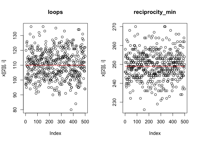
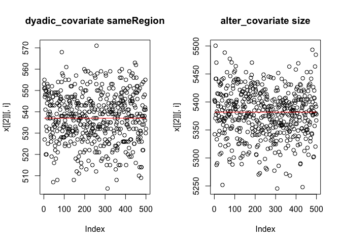
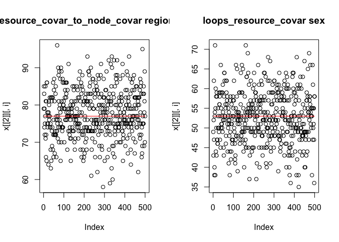
The output of extractTraces indicates the correlation of statistics between subsequent draws from the chain in phase 3. The plot should show data points randomly scattered around the target line, as shown below. If patterns in the traces are discernible, a higher thinning is needed.
Based on an estimated model, a score-type test is available that shows whether statistics representing non-included effects are well represented. If this is not the case, it is likely that including them will result in significant estimates.
myEffects2 <- createEffects(myState) |>
  addEffect(transitivity_min)

test_ME.2 <- scoreTest(myResDN, myEffects2)
test_ME.2
#> Results
#>            Effects pValuesParametric pValuesNonParametric
#> 1 transitivity_min      4.790818e-09                    0
#>
#>  Parametric p-values: small = more significant
#>  Non-parametric p-values: further away from 0.5 = more significant
The interpretation is that there appears to be some transitive clustering in the data that the model does not account for in its current form.
Akin to ERGMs, goodness of fit testing is available to see whether auxiliary statistics are well captured by the model.
myGofIndegree <- monanGOF(ans = myResDN, gofFunction = getIndegree, lvls = 1:70)
plot(myGofIndegree, lvls = 20:70)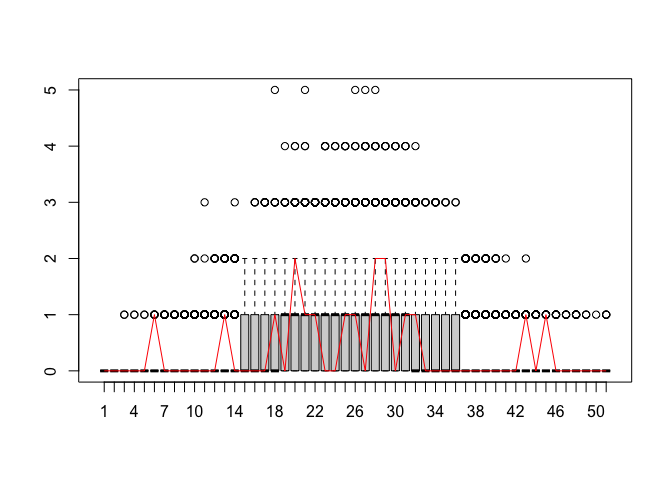
myGofTieWeight <- monanGOF(ans = myResDN, gofFunction = getTieWeights, lvls = 1:20)
plot(myGofTieWeight, lvls = 1:20)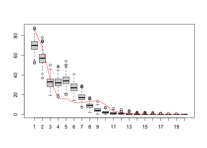
The package also provides the possibility to exemplarily simulate mobility networks based on the data and the specified effects and parameters.