![]()
![]()
The goal of cloneRate is to provide easily accessible methods for estimating the growth rate of clones. The input should either be an ultrametric phylogenetic tree with edge lengths corresponding to time, or a non-ultrametric phylogenetic tree with edge lengths corresponding to mutation counts. This package provides the internal lengths and maximum likelihood methods for ultrametric trees and the shared mutations method for mutation-based trees, all of which are from our recent paper cloneRate: fast estimation of single-cell clonal dynamics using coalescent theory. We also provide a birth-death Markov Chain Monte Carlo (MCMC) approach using the probability density derived in Eq. 5 of Tanja Stadler’s work.
To test our methods, we provide a fast way to simulate the coalescent (tree) of a sample from a birth-death branching process, which is a direct result of Amaury Lambert’s work.
Install from CRAN with the following:
install.packages("cloneRate")Alternatively, you can install the development version of cloneRate
from GitHub. For this basic tutorial
and our vignettes, we will also use a few other packages, which can all
be installed from CRAN. Because these are listed as packages we
‘suggest’, running the following command (with
dependencies = TRUE) will install them along with the
vignettes:
# Install devtools if you don't have it already
install.packages(setdiff("devtools", rownames(installed.packages())))

# Install
devtools::install_github("bdj34/cloneRate", build_vignettes = TRUE, dependencies = TRUE)
Alternatively, you can install them manually:
install.packages(setdiff(c("ggplot2", "ggsurvfit", "survival", "car"), rownames(installed.packages())))We’ll walk through simulating a single tree and plotting it. Then we’ll apply our growth rate methods.
We can simulate a sample of size n from a birth-death tree as follows:
library(cloneRate)
library(ape)
library(ggplot2)

# Generate a sampled tree with 100 tips from a 20 year birth-death process with birth rate a=1 and death rate b=0.5
tree <- simUltra(a = 1, b = 0.5, cloneAge = 40, n = 100)
Now that we have simulated the tree, let’s plot it:
# Plot, then add scale and title
plot.phylo(tree,
  direction = "downwards",
  show.tip.label = FALSE, edge.width = 2
)
axisPhylo(side = 2, backward = FALSE, las = 1)
title(main = "Simulated ultrametric tree", ylab = "Time (years)")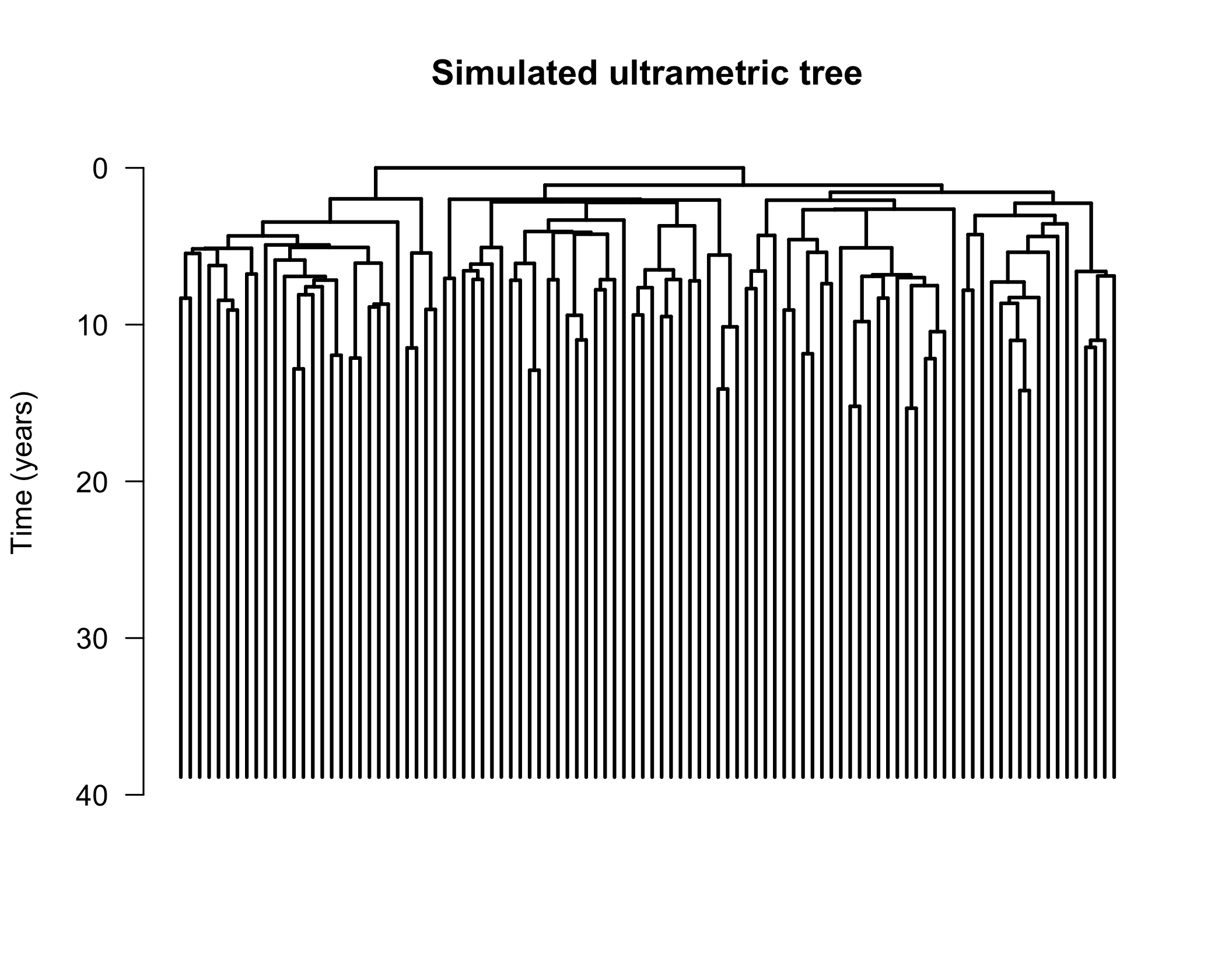
We can use this tree as input to our methods for growth rate estimation:
# Estimate the growth rate r=a-b=0.5 using maximum likelihood
maxLike.df <- maxLikelihood(tree)
print(paste0("Max. likelihood estimate = ", round(maxLike.df$estimate, 3)))
#> [1] "Max. likelihood estimate = 0.537"

# Estimate the growth rate r=a-b=0.5 using internal lengths
intLengths.df <- internalLengths(tree)
print(paste0("Internal lengths estimate = ", round(intLengths.df$estimate, 3)))
#> [1] "Internal lengths estimate = 0.527"
Because we’re simulating a new tree each time, the estimate will change with each run, so don’t be worried if your results don’t match exactly.
In our
paper, we use simulated trees to test our growth rate estimates. As
an example, let’s load some simulated data that comes with our package,
exampleUltraTrees has 100 ultrametric trees. In the
“metadata” data.frame we will find the ground truth growth rate, which
in this case is 1. Let’s apply our methods to all 100 trees.
# Here we are applying two methods to all of the ultrametric trees
resultsUltraMaxLike <- maxLikelihood(exampleUltraTrees)
resultsUltraLengths <- internalLengths(exampleUltraTrees)
Notice how the functions maxLikelihood() and
internalLengths() can take as input either a single tree or
a list of trees. Either way, the output is a data.frame
containing the results. Now that we have 100 estimates on 100 different
trees from 2 different methods, let’s plot the distributions
# Combine all into one df for plotting. This works because the columns are the same
resultsCombined <- rbind(resultsUltraMaxLike, resultsUltraLengths)

# Plot, adding a vertical line at r=1 because that's the true growth rate
ggplot(resultsCombined) +
  geom_density(aes(x = estimate, color = method), linewidth = 1.5) +
  geom_vline(xintercept = exampleUltraTrees[[1]]$metadata$r) +
  theme_bw() +
  theme(
    axis.text.y = element_blank(), axis.ticks.y = element_blank(),
    legend.title = element_blank()
  ) +
  xlab("Net growth rate estimate (r)") +
  ylab("Density") +
  scale_color_manual(labels = c("Internal lengths", "Max. likelihood"), values = c("black", "#009E73"))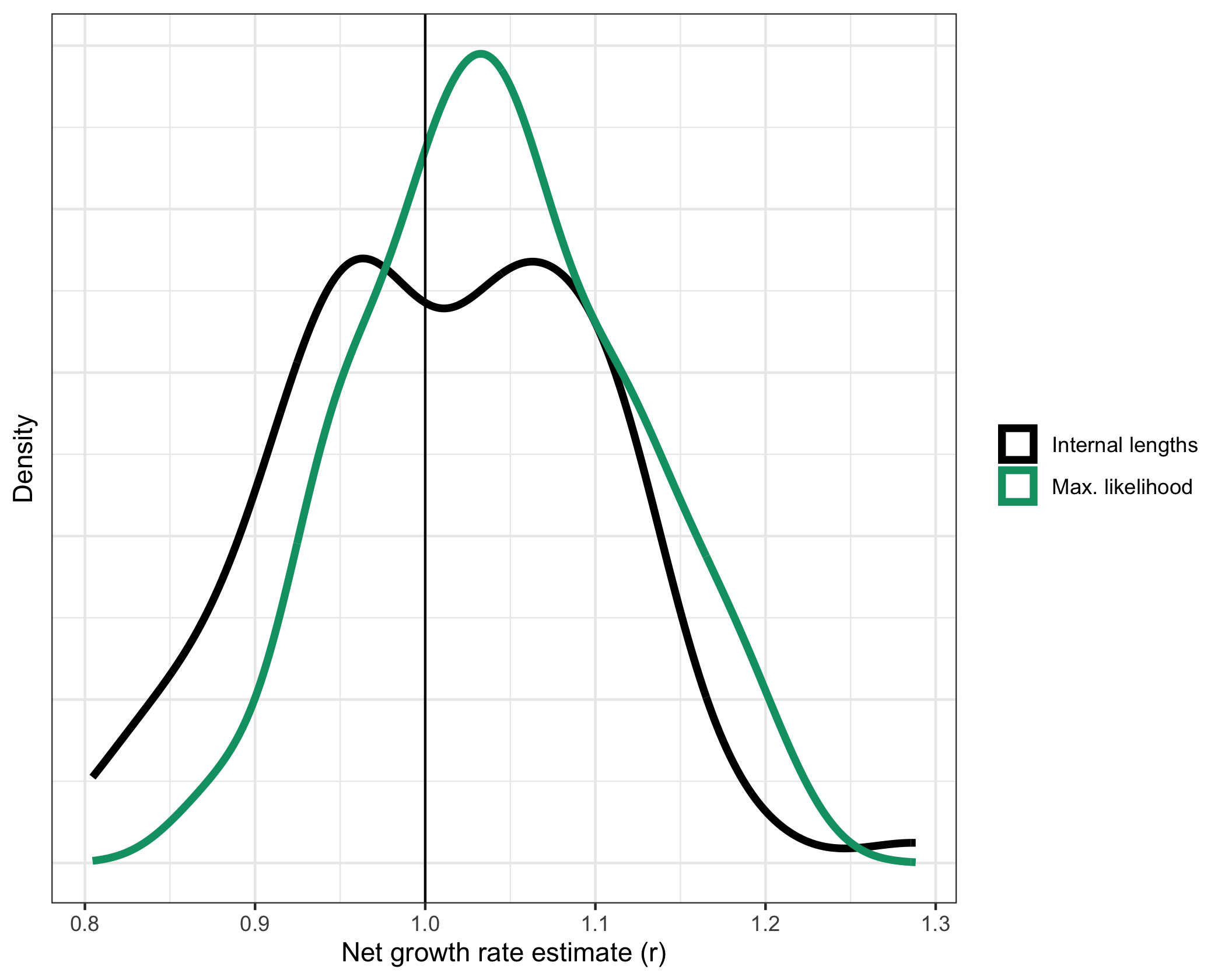
Finally, let’s compute the root mean square error (RMSE) of the estimates. We expect maximum likelihood to perform the best by RMSE, but 100 is a relatively small sample size so anything could happen…
# Calculate the RMSE
groundTruth <- exampleUltraTrees[[1]]$metadata$r[1]
rmse <- unlist(lapply(
  split(resultsCombined, resultsCombined$method),
  function(x) {
    sqrt(sum((x$estimate - groundTruth)^2) / length(x$estimate))
  }
))

print(rmse)
#>    lengths    maxLike
#> 0.09119116 0.08756432
As expected, maximum likelihood performs the best. Note that this may change if we regenerate the data. For more details, see the cloneRate website or vignettes:
vignette("cloneRate-dataAnalysis", package = "cloneRate")
vignette("cloneRate-simulate", package = "cloneRate")Simulating the birth-death trees is a direct result of the work of Amaury Lambert in:
Our package comes with 42 clones annotated from four distinct publications, which are the ones we use in our analysis. Note that there are three clones profiled at two different timepoints, meaning there are 39 unique clones. The papers which generate this data are:
The birth-death MCMC (not shown here) is based on the probability density derived in Eq. 5 of Tanja Stadler’s work:
The mathematical basis for our estimates is detailed in full in our paper.