ggincerta is an extension of ggplot2 for visualising
uncertainty in spatial data and, more generally, for constructing
bivariate visualisations. It reimplements the visualisation methods for
three map types introduced in the Vizumap package within
the grammar of graphics, while also providing additional uncertainty
visualisation approaches.
The package integrates directly with ggplot2 through custom scales, geoms, aesthetics, and guides. This allows uncertainty visualisations to be constructed, combined, and customised using the same workflow as conventional ggplot2 graphics.
# Install the release from CRAN:
install.packages("ggincerta")

# Install the development version from GitHub:
# install.packages("pak")
pak::pak("maggiexma/ggincerta")The example dataset included in ggincerta is an sf
object adapted from the nc shapefile in the sf
package. It contains two simulated variables, value and
sd, which are used throughout the examples to demonstrate
how regional estimates and uncertainty can be visualised
simultaneously.
For more details on the original visualisation designs implemented
from Vizumap, see https://doi.org/10.1002/sta4.150.
library(ggincerta)
#> Loading required package: ggplot2ggincerta provides scale_*_bivariate() for
constructing bivariate colour scales that can be used with
duo() inside ggplot2 aesthetics. Two variables are
discretised independently, and their crossed bin combinations are mapped
to a two-dimensional colour grid.
By default, automatically generated breaks use
breaks_pretty() on the transformed scale. The
n_breaks argument specifies the desired number of bins, but
when nice.breaks = TRUE, the actual number of bins may
differ in order to produce more readable break values.
ggplot(nc) + geom_sf(aes(fill = duo(value, sd)))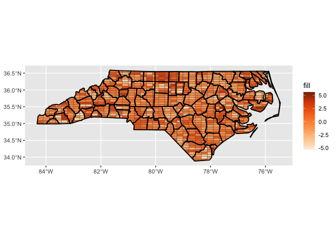
If an exact number of equal-width bins is required, set
nice.breaks = FALSE. Quantile-based binning is also
available by setting quantile = TRUE.
ggplot(nc) +
  geom_sf(aes(fill = duo(value, sd))) +
  scale_fill_bivariate(
    n_breaks = 4,
    nice.breaks = FALSE
  )
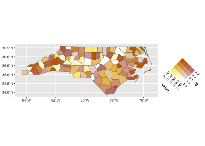
The default palette is generated by mixing two colour ramps.
Alternative palette functions can be supplied through
palette_fun. For example, bivar_fade_palette()
can be used to emphasise one variable while progressively suppressing
another perceptual dimension along the second axis.
ggplot(nc) +
  geom_sf(aes(fill = duo(value, sd))) +
  scale_fill_bivariate(
    palette_fun = bivar_fade_palette,
    colours = c("#F6E8C3", "orange", "red"),
    palette_params = list(fade = "desaturate")
  )
For complete control over the colour grid, ggincerta
also provides manual bivariate scales. Manual scales use exact
equal-width bins by default, so the number of required colours is
determined directly by n_breaks.
Value-Suppressing Uncertainty Palettes (VSUPs), proposed by Correll
et al. (2018), suppress value differences as uncertainty increases. In
ggincerta, they are implemented through
scale_*_vsup().
The uncertainty variable is divided into a hierarchy of layers, while the number of value bins varies across those layers according to the branch parameter. When breaks are not supplied, both value and uncertainty breaks are generated as equal-width intervals on the transformed scale.
ggplot(nc) +
  geom_sf(aes(fill = duo(value, sd))) +
  scale_fill_vsup()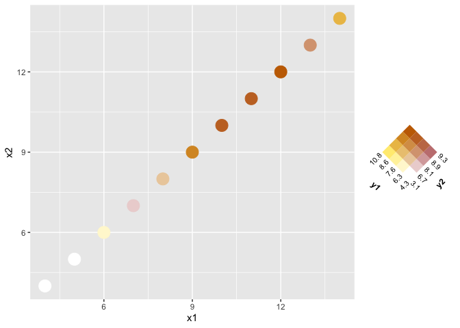
Custom breaks and limits can also be supplied explicitly.
ggplot(nc) +
  geom_sf(aes(fill = duo(value, sd))) +
  scale_fill_vsup(
    breaks = list(
      seq(-3, 3, length.out = 9),
      seq(0, 4, length.out = 5)
    ),
    limits = list(
      c(-3, 3),
      c(0, 4)
    )
  ) +
  theme(
    legend.text = element_text(size = 7)
  )
ggincerta provides geom_sf_pixel() for
constructing pixel maps. Each spatial unit is tessellated into pixels,
with pixel values sampled from a specified probability distribution
parameterised by the mapped variables.
Pixel grids can be generated using rectangular, square, or hexagonal cells, with hexagonal pixels used by default. Variation in pixel colours within a region provides a visual representation of uncertainty while retaining the spatial pattern of the underlying estimate.
Because pixel generation relies on geometric intersection, computation can be slower when working directly with geographic sf objects under the s2 geometry system. For improved performance, it is recommended to first transform the data to a projected planar coordinate reference system.
nc_flat <- sf::st_transform(nc, 3857)

ggplot(nc_flat) +
  geom_sf_pixel(
    mapping = aes(fill = duo_pixel(value, sd)),
    seed = 123
  )
The pixel shape and resolution can also be customised by
pixel_shape.
ggplot(nc_flat) +
  geom_sf_pixel(
    mapping = aes(fill = duo_pixel(value, sd)),
    pixel_shape = "square",
    n = 30,
    seed = 123
  )
Glyph maps use additional graphical marks placed at spatial centroids
to represent value and uncertainty. ggincerta provides
several glyph forms through geom_sf_glyph().
Regular shapes such as circles, squares, triangles, and hexagons can be used with bivariate colour scales.
ggplot(nc_flat) +
  geom_sf_glyph(
    mapping = aes(colour = duo(value, sd))
  )
#> Warning: st_point_on_surface assumes attributes are constant over geometries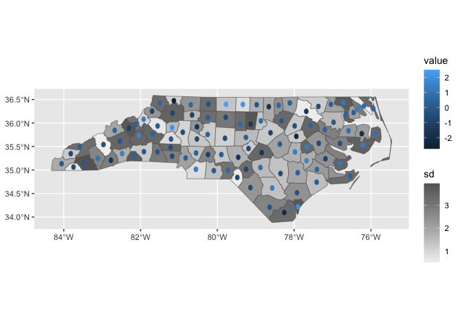
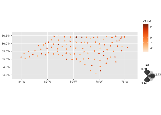
Drop-shaped glyphs provide an alternative encoding in which
uncertainty can be represented by rotation through the
angle aesthetic.
ggplot(nc_flat) +
  geom_sf_glyph(
    aes(colour = value, angle = sd),
    shape = "drop"
  )
#> Warning: st_point_on_surface assumes attributes are constant over geometries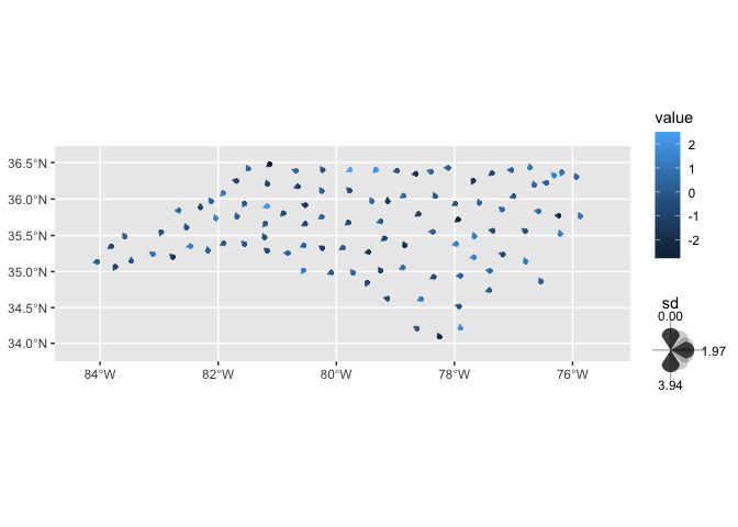
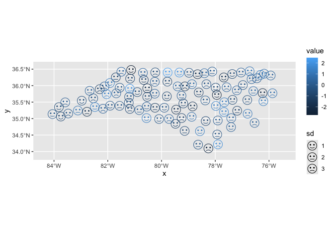
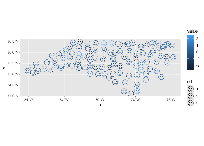
Chernoff faces provide another glyph form for multivariate encoding.
The implementation in ggincerta builds on the grob and
scale design provided by the ggChernoff package. In the
example below, facial colour represents the estimated value, while
facial expression represents uncertainty: lower uncertainty produces
smiling faces, whereas higher uncertainty produces frowning faces.
ggplot(nc_flat) +
  geom_sf_glyph(
    aes(colour = value, smile = sd),
    shape = "chernoff"
  )
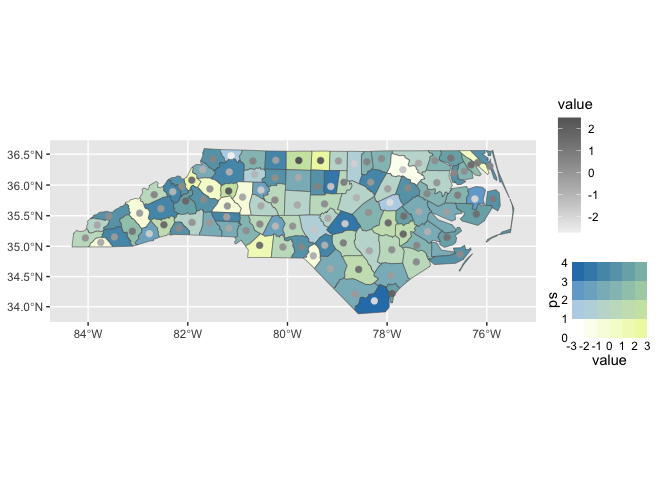
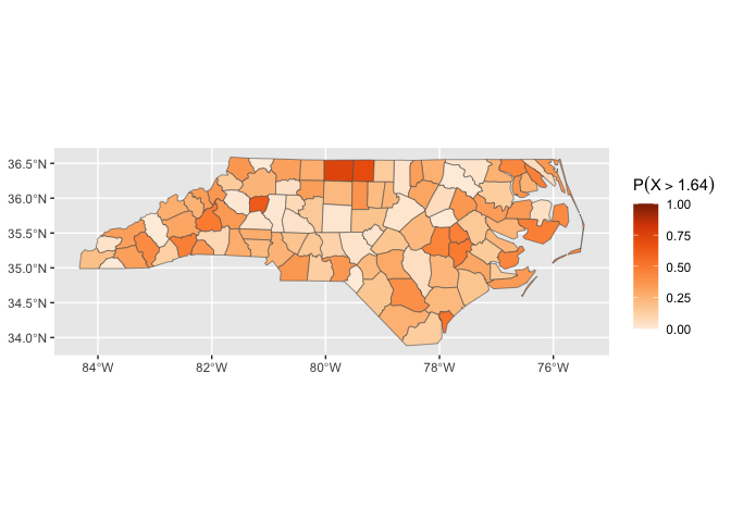
The dual map combines a conventional choropleth layer with a glyph layer in the same spatial display. The two layers can use separate aesthetics, scales, and guides, allowing the primary variable and uncertainty to remain visually distinct and directly interpretable.
A simple dual map can, for example, map uncertainty to polygon fill and the estimated value to glyph colour.
ggplot(nc_flat) +
  geom_sf_dualmap(
    aes(fill = sd, colour = value)
  )
#> Warning: st_point_on_surface assumes attributes are constant over geometries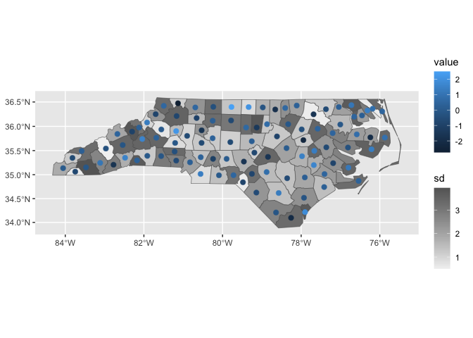
Because the choropleth and glyph components are layered within the
ggplot2 system, they can also be combined with bivariate mappings. This
makes it possible to encode an additional variable through
duo() while retaining a separate glyph-based
representation.
ggplot(nc_flat) +
  geom_sf_dualmap(
    aes(
      fill = duo(value, sd),
      colour = value
    )
  ) +
  scale_colour_gradient(low = "grey95", high = "grey40") +
  scale_fill_bivariate()
#> Warning: st_point_on_surface assumes attributes are constant over geometries