sobolnp

First-order Sobol sensitivity indices from the data you already have. sobolnp estimates how much of the variance of an output \(Y\) is explained by each input \(X_i\),

\[ S_i = \frac{\operatorname{Var}\left( \mathbb{E}[Y \mid X_i] \right)}{\operatorname{Var}(Y)}, \]

using only a sample of \((X, Y)\). It does not need to run the model again and does not need to know its formula.

Why sobolnp?

Most Sobol estimators are built for a computer model that you can call at will. They evaluate it on a specially designed set of points, usually many times. That is a problem when each model run is expensive, when the model is a black box you can no longer run, or when all you have is observational data.

	Monte Carlo / pick-freeze (Sobol, Saltelli, Jansen, …)	FAST	Metamodel (splines, kriging)	sobolnp
Needs to run the model	yes	yes	to train it	no
Needs a designed sample	yes (frozen copies)	yes (frequency design)	yes (training design)	no, any i.i.d. sample
Model runs typically needed	\(10^4\)–\(10^5\)	\(10^3\)–\(10^4\)	\(10^2\)–\(10^3\) + fitting	the sample you have (\(10^2\)–\(10^3\))
Finite-sample bias correction	—	—	depends on the metamodel	bootstrap reduces the CV bias

sobolnp is a good fit when:

you only have a data set, or the model is too expensive to evaluate again;
the relation between inputs and output is unknown and possibly strongly non-linear;
you want two complementary estimates (CV and bootstrap) instead of a single smoother with a default bandwidth.

In the reference paper (Solís 2021), 1,000 observations of a hydraulic dyke model gave the same ranking of inputs as classic Monte Carlo estimates based on \(10^5\) model runs, with similar values for the dominant inputs.

Other estimators that work from given data exist, for example the rank- and nearest-neighbour-based estimators in the sensitivity package. What sobolnp adds is a smooth non-parametric fit of every \(\mathbb{E}[Y \mid X_i]\) together with a bandwidth chosen to reduce the bias of the index.

How it works

Fit. For each input, \(\mathbb{E}[Y \mid X_i]\) is estimated by kernel (Nadaraya–Watson) regression with an Epanechnikov kernel, using np. The index is the variance of the fitted curve divided by the variance of \(Y\).
CV bandwidth. The bandwidth is first chosen by least-squares cross-validation. It works asymptotically, but in finite samples it over-smooths and tends to underestimate \(S_i\).
Bootstrap bandwidth. The residuals of the CV fit are rescaled and resampled to build nboot bootstrap responses. For a candidate bandwidth, the bootstrap fits measure how much smoothing flattens the curve, and that amount is added back to the CV curve. The bandwidth is searched below the CV bandwidth, and the resulting index is reported as the bootstrap estimate.

sobolnp() reports both estimates, so you can see how much the correction matters for each input.

Example

The g-Sobol function is a standard, strongly non-linear benchmark with known indices:

\[ Y = \prod_{i=1}^{4} \frac{|4X_i - 2| + a_i}{1 + a_i}, \qquad X_i \sim \mathcal{U}(0, 1),\quad a = (0, 1, 4.5, 9). \]

library(sobolnp)

a <- c(0, 1, 4.5, 9)
g_sobol <- function(X) {
  apply(X, 1, function(x) prod((abs(4 * x - 2) + a) / (1 + a)))
}

set.seed(123)
X <- matrix(runif(4 * 1000), ncol = 4)
Y <- g_sobol(X)

estimation <- sobolnp(Y = Y, X = X, nboot = 100, verbose = FALSE)
estimation
#> 
#> Call:
#> sobolnp(Y = Y, X = X, nboot = 100, verbose = FALSE)
#> 
#> Number of observations: 1000 
#> Number of variables: 4 
#> 
#> First order indices
#>        Si CV   bw CV Si Bootstrap bw Bootstrap
#> X1 0.6705288 0.03226     0.700250     0.001465
#> X2 0.1887558 0.04239     0.196459     0.004435
#> X3 0.0174166 0.08971     0.019063     0.009809
#> X4 0.0006614 0.18639     0.001178     0.034906

Compared with the exact values:

V <- 1 / (3 * (1 + a)^2)
round(cbind(exact = V / (prod(1 + V) - 1),
            CV = estimation$S,
            bootstrap = estimation$Sboot), 3)
#>    exact    CV bootstrap
#> X1 0.716 0.671     0.700
#> X2 0.179 0.189     0.196
#> X3 0.024 0.017     0.019
#> X4 0.007 0.001     0.001

plot(estimation)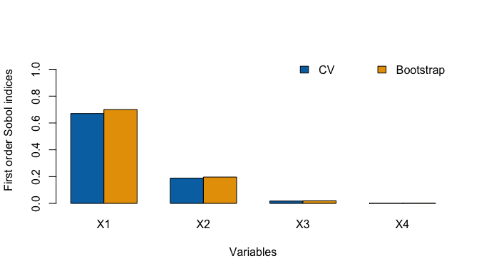

Reading the results

Ranking first. Both estimates usually agree on which inputs matter. This is the most reliable output.
CV below, bootstrap closer. For influential inputs, the CV estimate tends to fall below the true index. In simulations with the default kernel (g-Sobol, Ishigami and an additive model with noise, \(n = 300\)), the bootstrap estimate reduced that bias and had a lower average error than CV, although on individual samples CV is sometimes closer.
Kernel order. With ckerorder = 4 the CV estimate is already less biased, and the bootstrap correction can overshoot. The default (ckerorder = 2) is the recommended setting.
Non-influential inputs. When \(\mathbb{E}[Y \mid X_i]\) is flat, the selected bandwidth becomes very large and \(S_i \approx 0\). This is the expected result, not a failure.
Scope. Only first-order indices are estimated. Interaction and total indices are not. Weak or very irregular effects can be underestimated.

Main arguments

Argument	Default	Purpose
`nboot`	`100`	Bootstrap samples. More is more stable and slower.
`bootstrap`	`TRUE`	`FALSE` returns only the fast CV estimates.
`ckerorder`	`2`	Kernel order (2, 4, 6 or 8).
`bandwidth`, `bandwidth.compute`	`NULL`, `TRUE`	Starting bandwidths, or fixed ones with `bandwidth.compute = FALSE`.
`mc.cores`	`1`	Inputs processed in parallel (Unix-alikes).
`verbose`	`TRUE`	Progress messages and bars.

The cost grows with the number of inputs × nboot. For a first look at many inputs, run with bootstrap = FALSE, then bootstrap the relevant ones.

Installation

# From CRAN
install.packages("sobolnp")

# Development version
# install.packages("pak")
pak::pak("maikol-solis/sobolnp")

Citation

If you use sobolnp, please cite (also available with citation("sobolnp")):

Solís, M. (2021). Non-parametric estimation of the first-order Sobol indices with bootstrap bandwidth. Communications in Statistics - Simulation and Computation, 50(9), 2497–2512. https://doi.org/10.1080/03610918.2019.1655575